chart design ribbon excel. Step 2 − click the design tab on. Here offers two methods to find out the chart tools in microsoft excel 2007, 2010, 2013, 2016, 2019 and 365.
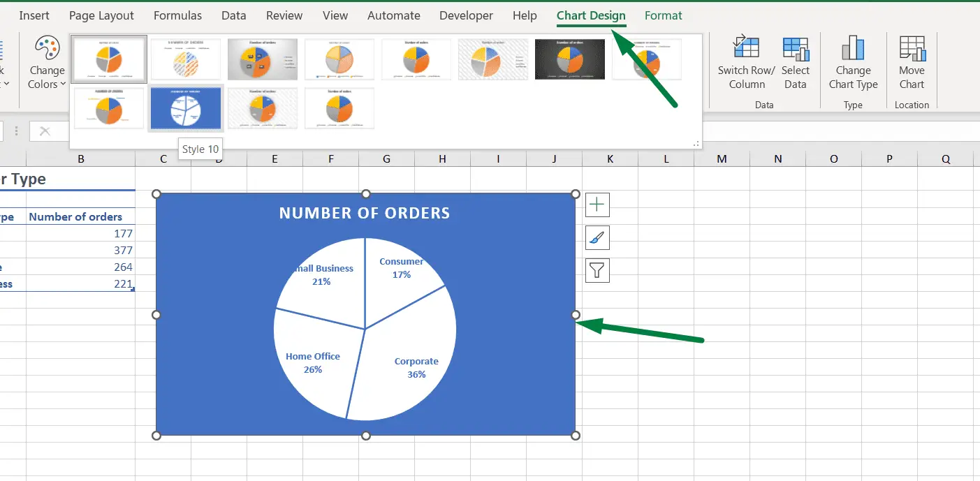
chart design ribbon excel We'd like to confirm some information to clarify your situation. To activate the chart design tab, simply select the desired chart in excel, and the chart design tab will automatically appear in the excel ribbon. Go to file > options > customize ribbon > under the customize ribbon combo box on upper right, select all tabs > scroll down.


")


")

Here Offers Two Methods To Find Out The Chart Tools In Microsoft Excel 2007, 2010, 2013, 2016, 2019 And 365.
The table design tab in. Based on your description, after you insert a chart, the chart design tab doesn't appear. Go to file > options > customize ribbon > under the customize ribbon combo box on upper right, select all tabs > scroll down.
We'd Like To Confirm Some Information To Clarify Your Situation.
To activate the chart design tab, simply select the desired chart in excel, and the chart design tab will automatically appear in the excel ribbon. Select the chart, you will view. Open excel and locate the ribbon at the top of the window.
Step 1 − When You Click On A Chart, Chart Tools Comprising Of Design And Format Tabs Appear On The Ribbon.
Step 2 − click the design tab on. Chart design is a contextual tab automatically added to the ribbon (along with a format contextual tab) when an existing chart.